
Pairs trading strategy is a market neutral strategy that involves the following two steps.
The first step is to identify pairs, which are trading instruments (stocks, options, currencies, bonds, etc.) that show high correlations, i.e., the price of one moves in the same direction as the other. In the second step, pairs traders look for divergence in prices between a pair. When a divergence is noted, traders take opposite positions for instruments in a pair. In this study, we examine a pairs trading strategy based on publicly traded common equity. In equity-pairs trading, the trader takes the long position for underperforming stocks and the short position for over performing stocks. The trader then profits from the correction of the divergence.
We test an equity pairs trading strategy that uses historical return correlations to determine pairs. We first estimate the pairwise stock return correlations for all the Center for Research in Security Prices (CRSP) firms for each year using return data from the previous five years. For each stock, we identify a set of pair stocks that tend to move most closely with that stock in the last five years. If a given stock’s return deviates from its pair stocks in a given month, we examine whether its return converges to its pair stocks in the future and provides a potential trading opportunity. We find that a trading strategy that bets on this convergence generates six-factor (market, size, book-to-market, momentum, short-term reversal, and liquidity) alphas of up to 9% annually for a value-weighted self-financing portfolio, and 36% for an equal-weighted portfolio. In addition, our pairs trading profits cannot be explained by investment-based factors, funding liquidity risk or financial intermediary leverage factor. The proposed pairs residual is also different from existing residual type return predictors.
Our return difference variable is essentially the difference between pairs return and lagged stock return. Thus, the pairs trading profits must stem from the pairs momentum and/or the short-term reversal. We further examine which one of these components is driving the pairs returns profits and whether the two components have similar properties. We find that the short-term reversal explains part of the pairs trading strategy returns. However, there are still substantial returns to the pairs trading strategy even when there is no significant movement in a firm’s stock but its pairs have experienced significant price changes, i.e., a stock converges to its pairs even when there is no shortterm reversal per se. Therefore, both the short-term reversal and the pairs momentum contribute to the pairs trading profits. We also find that the short-term reversal and pairs momentum components have different dynamic and cross-sectional properties. Specifically, the profits to pairs momentum is basically zero after the first month. However, the profits to short-term reversal reverse after the first month. We also find that the profits to the short- term reversal strategy are larger in stocks that are in a poorer information environment and more illiquid, however profits to the pairs momentum strategy appear largely unrelated to information environment and liquidity in the cross section. We conclude that while information diffusion and liquidity provision may help explain the pairs trading, there may be other economic channels at work.
Given that the short-term reversal is relatively well studied, we further study what explains our pairs momentum. We find that it is largely explained by the onemonth version of the industry momentum. For example, in a double sorting procedure, after we control for the lagged one month industry return, the difference between the lagged pairs return and industry return generates an average of 0.29% monthly return differential in the value-weighted portfolios. On the other hand, after we control for the difference between the lagged pairs return and industry return, the lagged one month industry return generates an average of 0.7% return differential per month. We also find that the conventional six-month industry momentum in Moskowitz and Grinblatt (1999) concentrates in the first month, coinciding with the return horizon of pairs momentum.
Profitability of a Pairs Trading Strategy
In this section, we propose and test an equity pairs trading strategy based on the historical pairwise return correlations. Essentially, this test examines whether the information in stock comovement is fully impounded into the prices.
We identify the pairs portfolio as follows. For each stock i in year t + 1, we compute the Pearson correlation coefficients between the returns of stock i and all other stocks in the CRSP using monthly data from January of year t − 4 to December of year t. We then find 50 stocks with the highest correlations to stock i as its pairs.1 In each month in year t + 1, we compute the pairs portfolio return as the equal-weighted average return of the 50 pairs stocks, Cret. Our pairwise trading hypothesis is that if in any given month in year t + 1, a stock’s return, Lret, deviates from its pairs portfolio returns, Cret, then in the following month this divergence should be reversed. For example, if a stock significantly underperforms its pairs portfolio, that stock should experience abnormally higher returns in the next month :
RetDiff betaс ∗ (Cret-Rf) − (Lret−Rf),
Where Rf is the risk-free rate and betaс is the regression coefficient of firm i’s monthly return on its pairs portfolio return using monthly data between year t −4 and t. The use of betaс addresses the issue of different return volatilities between the stock and its pairs portfolio.
For n stocks, there are n ∗ (n − 1)/2 correlations to be computed. Because the number of observations for the correlations grows exponentially with the number of stocks, the estimation is computationally intensive. To reduce the computation burden, we require that all firms have 60 monthly stock returns data from year t −4 to year t.
Table 1 reports the returns of the portfolios sorted on RetDiff. In each month, we form 10 portfolios, Decile 1 through Decile 10, based on the previous month’s RetDiff; the holding period is one month. Note that while the return difference between a portfolio of 50 most-highly correlated stocks with stock i and stock i is used as a sorting variable, only individual stock i enters the portfolio construction, not those 50 stocks. The portfolio of those 50 stocks only serves as a benchmark for portfolio sorting. Our sample period is from January 1931 to December 2007. In panel A, we report raw returns, Fama–French three factor (market, size, and book-to-market) alphas, five factor (the three factors plus momentum and short-term reversal factors) alphas, and six-factor (the three factors plus momentum, short-term reversal, and liquidity factors) alphas for the value-weighted portfolios. We use the short-term reversal factor to examine the pairs trading strategy returns because by construction, the sorting variable RetDiff holds information from a stock’s lagged returns. The liquidity factor is the Pastor-Stambaugh value-weighted traded liquidity factor, which we include to examine the possibility that the RetDiff sorted portfolios compensate for liquidity provision.
An examination of the raw returns and alphas of the decile portfolios shows that stocks with high RetDiff have higher subsequent returns. For the value weighted portfolios, the zero-cost portfolio Decile 10 − Decile 1 (i.e., longing Decile 10 and shorting Decile 1) generates a return of 1.40% per month (t = 8.81). Unless stated otherwise, all t-statistics are Newey– West adjusted. The hedge portfolio has a three-factor adjusted alpha of 1.23% with a t-value of 7.69 and a six-factor adjusted alpha of 0.77% (t = 3.75). In addition to the significant hedge portfolio alphas, the alphas increase almost monotonically from Decile 1 to Decile 10, indicating that sorting on RetDiff systematically drives the hedge portfolio returns.
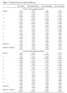
Notes: This table reports the value- and equal-weighted returns for portfolios that we form on the return difference (RetDiff ). Cret is the previous month’s pairs portfolio return. For each month in year t + 1, the pairs portfolio is the equal-weighted portfolio of the 50 stocks with the highest return correlations to a given stock between year t − 4 and year t. Lret is the previous month’s stock return. RetDiff is betac ∗(Cret-Rf) − (Lret − Rf), where betac is the regression coefficient of a firm’s monthly return on its pairs portfolio return in the most recent five years. The three factors are excess market return, small minus big (SMB), and high minus low (HML). The five factors are the three factors, the momentum factor, and the short-term reversal factor. The six factors are the five factors, plus Pastor-Stambaugh’s liquidity factor. Panel A reports value-weighted portfolios formed using all stocks with 60 monthly returns in the last five years. Panel B reports equal-weighted portfolios formed using all stocks with 60 monthly returns in the last five years. Monthly returns and alphas are reported in percentage with Newey–West six-lag adjusted t-statistics in parentheses. The sample period is from January 1931 to December 2007, except for the six-factor alphas (from January 1968 to December 2007).
The equal-weighted portfolios generate even higher dispersion in returns. Panel B of Table 1 reports the raw returns, three-factor alphas, five-factor alphas, and six-factor alphas for equal-weighted portfolios sorted by RetDiff. For the equal-weighted portfolios, the zero cost portfolio Decile 10−Decile 1 (i.e., longing Decile 10 and shorting Decile 1) generates a return of 3.59% per month (t 12.57). The three-factor alpha for the self-financing portfolio is 3.17% per month (t 13.75). The six-factor alpha is 3.03% (t = 13.35). Overall, the results in Table 1 suggest that the pairs trading strategy generates significant abnormal returns.
Figure 1 plots the annual returns of the value weighted (top panel) and equal-weighted (bottom panel) hedge portfolios based on the pairs trading strategy from 1931 to 2007. The value-weighted hedge portfolio generates negative returns in 12 years (1941, 1957, 1973, 1981, 1993, 1996, 1999, 2000, 2001, 2003, 2005, and 2007). By contrast, the equal-weighted hedged portfolio generates returns that are greater and only lost money in one year (−9.35% in 2007).
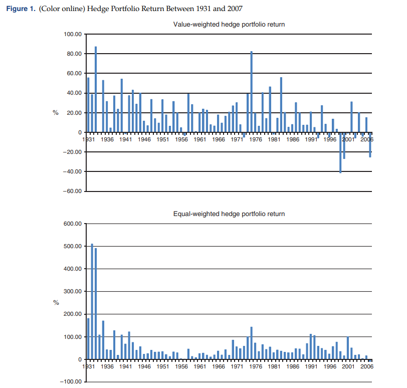
Notes: This figure plots the value-weighted (top panel) and equal-weighted (bottom panel) self-financing portfolio (Decile 10−Decile 1) returns for the portfolios that are formed on return difference (RetDiff ). Cret is the previous month’s pairs portfolio return. For each month in year t +1, the pairs portfolio is the equal-weighted portfolio of the 50 stocks with the highest return correlations to a given stock between year t −4 and year t. Lret is the previous month’s stock return. RetDiff is betac∗ (Cret-Rf) − (Lret − Rf), where betac is the regression coefficient of a firm’s monthly return on its pairs portfolio return in the most recent five years. The sample period is from 1931 to 2007.
Can Pairs Trading Be Explained by Common Risk Factors?
Table 1 shows that the pairs trading strategy returns survive the six-factor model, hence they are unlikely to be explained by common risk factors. We now investigate this possibility further by examining the risk factor loadings and the cross-sectional regressions. We first examine the factor-loadings of the pairs based decile portfolios to investigate how the pairs portfolios correlate with these common factors. Table 2 reports the loadings of the pairs portfolios with respect to the six factors, i.e., market, size, book-to-market, momentum, short-term reversal, and liquidity factor.
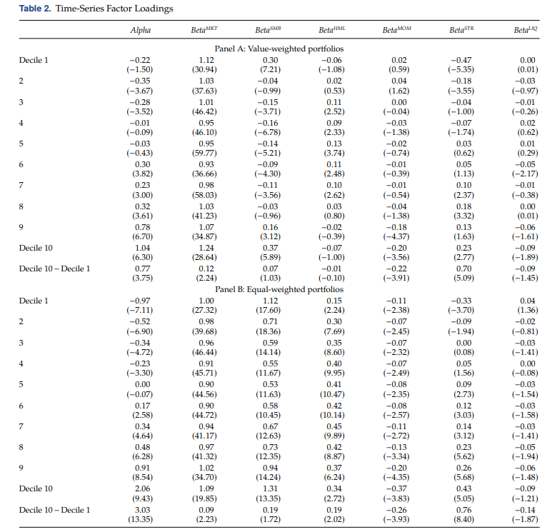
Notes: This table reports the factor loadings for portfolios that we form on the return difference (RetDiff ). Cret is the previous month’s pairs portfolio return. For each month in year t + 1, the pairs portfolio is the equal-weighted portfolio of the 50 stocks with the highest return correlations to a given stock between year t − 4 and year t. Lret is the previous month’s stock return. RetDiff is betac∗ (Cret-Rf) − (Lret − Rf), where betac is the regression coefficient of a firm’s monthly return on its pairs portfolio return in the most recent five years. The six factors are the excess market return, SMB, HML, the momentum factor, the short-term reversal factor, and Pastor and Stambaugh’s (2003) liquidity factor. Newey–West six-lag adjusted t-statistics are reported in parentheses. The sample period is from January 1968 to December 2007.
For the value-weighted portfolios (panel A), the self-financing portfolio (Decile 10 − Decile 1) loads positively and significantly on the market excess returns and the short-term reversal, and negatively and significantly on the momentum factor, but its loadings on SMB, HML, and liquidity factor are economically and statistically insignificant. The market beta increases with RetDiff, but this increase is not monotonic and the difference in beta is relatively small (1.13 in Decile 1 versus 1.24 in Decile 10). The pairs trading profits are negatively correlated with momentum beta, suggesting that the momentum factor cannot explain the pairs trading profits. The loading on the Pastor-Stambaugh traded liquidity factor is insignificant and slightly negative, suggesting that the pairs trading strategy is unlikely to be explained by compensation for systemic liquidity provision. Among these factors, the loading on the short-term reversal factor (ST_Rev) is positive and significant (0.70 with a t-statistic of 5.09) and the magnitude is larger and more significant than the loadings on the other factors. The results based on the equal-weighted portfolios (panel B) are similar: The self-financing portfolio loads positively on the market, SMB, HML, and especially short-term reversal and loads negatively on the momentum factor and liquidity factor. The beta on the short-term reversal factor is larger and more significant compared with the betas on the other factors.
The positive loading of the pairs trading hedge portfolio on the short-term reversal mimicking portfolio suggests that the strategy partially captures the short-term reversal phenomenon. However, the fact that the pairs trading portfolios still generate significant alphas after controlling for the short-term reversal factor and the other common factors (Table 1) suggests that the pairs trading strategy is not completely driven by the short-term reversal of a firm’s stock returns. We further examine the relation between short-term reversal and pairs trading in Section 3.
We also examine the relation between pairs trading with common risk factors using a cross-sectional regression approach. Table 3 reports the Fama–MacBeth regressions of monthly returns on the previous month’s pairs-portfolio return, Cret; the firm’s own return in the previous month, Lret; and other control variables. For returns between July of year t +1 and June of year t +2, we match with size and book-to-market equity at the fiscal year end in year t. For the market value of equity, we use Compustat total shares outstanding multiplied by the fiscal year-end price. Size is the logarithm of the market value of equity. We construct the book value of equity as total assets minus total liabilities. Book-tomarket equity is then the logarithm of the ratio of the book equity to the market value of equity. Momentum is the cumulative return over month −12 to month −2.
The Amihud measure is calculated using daily return and volume within a month (Amihud 2002). Henceforth, the coefficients on the Amihud measure are multiplied by 106 for readability. Idiosyncratic volatility is estimated with respect to the Fama–French threefactor model using daily return within a month (Ang et al. 2006). MAX is the maximum daily return within a month (Bali et al. 2011). BetaMKT , BetaSMB , BetaHML , and BetaMOM are estimated using monthly returns over the past 60 months. Because of the data availability in Compustat, these regressions are for the sample period from July 1951 to December 2007. We report the time-series average of cross-sectional regression coefficients with Newey–West six-lag adjusted t-statistics in parentheses.
Columns 1 and 2 in Table 3 show that, consistent with the portfolio results in Table 1, RetDiff positively predicts next month’s return, and that the effect is highly statistically significant, even after we include other return determinants (the coefficient on RetDiff in column 2 is 0.080 with a t-statistic of 18.01). To examine whether the pairs trading abnormal returns are incremental to those of the short-term reversal strategy, we split RetDiff into its two components (Cret and Lret) and include them directly in the regressions. We find that Cret predicts returns positively and Lret predicts returns negatively. In column 3, the coefficient on Cret is 0.226 (t 13.18) and that on Lret is −0.068 (t −15.72). The fact that Cret is statistically significant even when Lret is included in explaining future returns suggests that there is information in the pairs stocks that is not driven by just the short-term reversal phenomenon. In column 4, we add control variables to the regression. The coefficients on Cret and Lret remain statistically significant. In the last two columns, we examine the cross-sectional predictive power of Cret and Lret separately with control variables. Results suggest that both pairs return effect (coefficient = 0.090, t = 7.07) and short-term reversal effect (coefficient = −0.072, t = −16.35) contribute to the pairs trading profit.
Other Possible Explanatory Factors of Pairs Trading Profits
While Table 1 indicates that returns of the pairs trading strategy are not absorbed by commonly used risk factors, it is possible that the pairs trading portfolio can be explained by other pricing models. We explore two possible explanations that could result in pairs trading profits in Table 4.
The first model we consider is the Q-factor model proposed by Hou et al. (2015, 2017). Panel A of Table 4 presents the time-series regression results. The four factor (MKT, ME, I/A, and ROE) model cannot explain the pairs trading profits: Monthly alphas are 0.94% (t = 2.81) and 3.40% (t9.71) for value-weighted and equal-weighted Decile 10 − Decile 1 hedged portfolios, respectively. Pairs trading portfolios have positive and significant loadings on the market factor. The equal weighted portfolio has negative and significant loading on the ROE factor (BetaROE = −0.45, t = −3.15). Nevertheless, the alphas are similar to those in Table 1. Overall, the results suggest that the Q-factor model is not the underlying driving force of pairs trading returns.
The second possible explanation is financial friction that might affect arbitrageurs’ ability to exploit pairs trading profits. For example, time-varying funding liquidity risk or financial intermediary’s leverage could have an impact on arbitrage capital and therefore explain pairs trading profits over time. We look into this possibility in panels B and C of Table 4. Panel B reports the time-series regression results when funding liquidity risk is used to explain the Decile 10 − Decile 1 hedge portfolios. Funding liquidity risk is proxied by investment banks’ excess returns as in Ang et al. (2011). We find that returns of pairs trading portfolios remain after we use investment banks’ excess return in the time-series regressions. Monthly alphas range from 0.87% for the value-weighted portfolio to 2.98% for the equal-weighted portfolio. These alphas are similar to those in Table 1. The loadings on the funding liquidity risk are also small, ranging from 0.02 to 0.14. These results suggest that funding liquidity is not the main drive for the pairs trading profits.
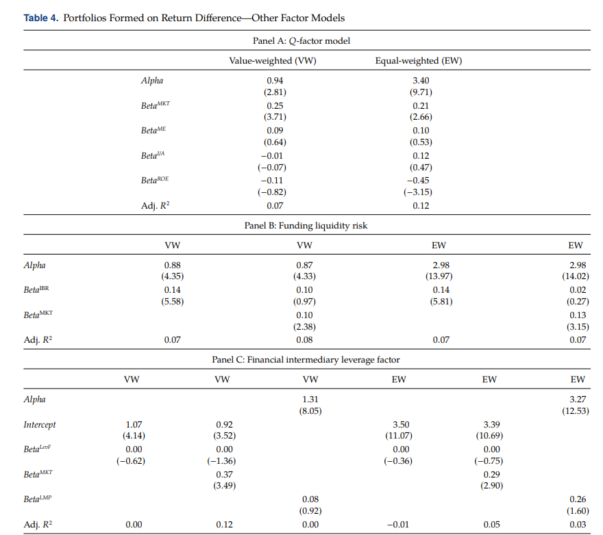
Notes: This table reports the value- and equal-weighted returns for portfolios that we form on the return difference (RetDiff ). Cret is the previous month’s pairs portfolio return. For each month in year t + 1, the pairs portfolio is the equal-weighted portfolio of the 50 stocks with the highest return correlations to a given stock between year t − 4 and year t. Lret is the previous month’s stock return. RetDiff is betac ∗(Cret-Rf) − (Lret − Rf), where betac is the regression coefficient of a firm’s monthly return on its pairs portfolio return in the most recent five years. Panel A reports alphas and betas of the value-weighted and equal-weighted Decile 10 − Decile 1 hedged portfolios against the “Q-theory” based factors. ME is the market equity, I/A is the investment-to-assets, and ROE is the return-on-equity. The sample period is from January 1967 to December 2007. Panel B reports alphas and betas of the value-weighted and equal-weighted Decile 10 − Decile 1 hedged portfolios against the funding liquidity risk. The proxy for the funding liquidity risk is investment banks’ excess returns (IBR). The sample period is from February 1962 to December 2007. Panel C reports alphas and betas of the value-weighted and equal-weighted Decile 10−Decile 1 hedged portfolio against the financial intermediary leverage factor. The sample period is from the first quarter of 1968 to the fourth quarter of 2007 for the original financial intermediary leverage factor, LevF, and from January 1931 to December 2007 for the factor mimicking portfolio, LMP. Alphas are presented in monthly percentage with Newey–West four-lag adjusted t-statistics in parentheses.
In panel C of Table 4, we adopt financial intermediary’s leverage factor in the time series regression. Results indicate that intermediary’s leverage is not the main driver for pairs trading profits: The slope coefficient on the intermediary’s leverage is basically 0. As the original leverage factor is not traded and only available at quarterly frequency, we use a traded leverage factor (LMP) and redo the exercise. The beta coefficient on the tradable leverage factor is 0.08 for the value-weighted hedged portfolio and 0.26 for the equal-weighted hedged portfolio. The alphas are 1.31% per month for the value-weighted portfolio and 3.27% per month for the equal-weighted portfolio, similar to those in Table 1. Taken together, while financial friction such as arbitrage capital might partially help explain pairs trading profits, it is not the key driver.
In the online appendix, we also consider whether conditional capital asset pricing model (CAPM) can explain the return spread of RetDiff sorted portfolios. We select four information variables, including the lagged T-bill rate, lagged dividend yield on the stock market, lagged yield spread between ten-year Treasury bond and three-month T-bill, and lagged yield spread between Moody’s BAA and AAA bonds. We find that beta loadings conditional on those information variables cannot explain the return difference across RetDiff sorted portfolios (see Table A.1).
The other possibility is that our results are caused by microstructure induced noises. To examine this possibility, we construct the RetDiff sorted portfolios using stocks with price greater than $5 and size greater than 10% NYSE cutoff. We find that the hedged value- and equal-weighted portfolios still earn positive and significant returns (see Table A.2).
After the first draft is written, we have also extended the sample period to over the 2008–2015 period. This constitutes a true out-of-sample test. We find that the trading profits have declined in the recent sample period. However, the hedged portfolios are still statistically and economically significant for the equal weighted portfolios (see Table A.4).